Quantum Wave in a Box app for iPhone and iPad

Schrödinger equation solver 1D. User defined potential V(x). Diagonalization of hamiltonian matrix. Animation showing evolution in time of a gaussian wave-packet.

In Quantum Mechanics the one-dimensional Schrödinger equation is a fundamental academic though exciting subject of study for both students and teachers of Physics. A solution of this differential equation represents the motion of a non-relativistic particle in a potential energy field V(x). But very few solutions can be derived with a paper and pencil.

Have you ever dreamed of an App which would solve this equation (numerically) for each input of V(x) ?

Give you readily energy levels and wave-functions and let you see as an animation how evolves in time a gaussian wave-packet in this particular interaction field ?

Quantum Wave in a Box does it ! For a large range of values of the quantum system parameters.

Actually the originally continuous x-spatial differential problem is discretized over a finite interval (the Box) while time remains a continuous variable. The time-independent Schrödinger equation H ψ(x) = E ψ(x), represented by a set of linear equations, is solved by using quick diagonalization routines. The solution ψ(x,t) of the time-dependent Schrödinger equation is then computed as ψ(x,t) = exp(-iHt) ψ₀(x) where ψ₀(x) is a gaussian wave-packet at initial time t = 0.

You enter V(x) as RPN expression, set values of parameters and will get a solution in many cases within seconds !

- Atomic units used throughout (mass of electron = 1)
- Quantum system defined by mass, interval [a, b] representing the Box and (real) potential energy V(x).
- Spatially continuous problem discretized over [a, b] and time-independent Schrödinger equation represented by a system of N+1 linear equations using a 3, 5 or 7 point stencil; N being the number of x-steps. Maximum value of N depends on device’s RAM: up to 4000 when computing eigenvalues and eigenvectors, up to 8000 when computing eigenvalues only.
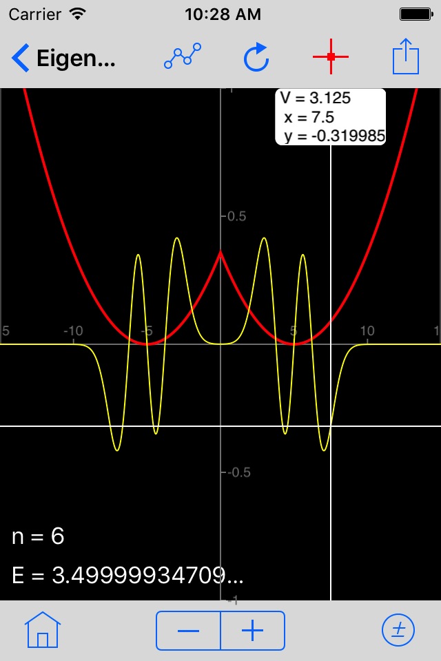
- Diagonalization of hamiltonian matrix H gives eigenvalues and eigenfunctions. When computing eigenvalues only, lowest energy levels of bound states (if any) with up to 10-digit precision.
- Listing of energy levels and visualisation of eigenwave-functions.
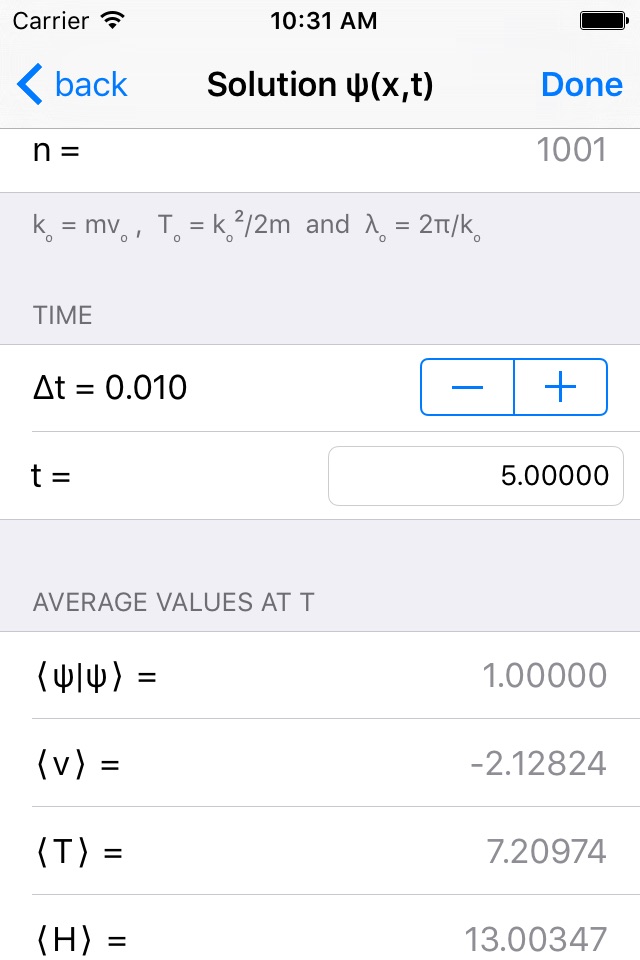
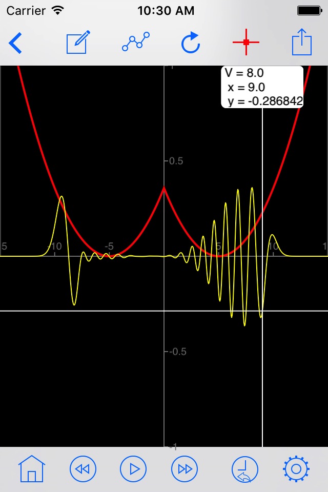
- Animation shows gaussian wave-packet ψ(x,t) evolving with real-time evaluation of average velocity, kinetic energy and total energy.
- Toggle between clockwise and counter-clockwise evolution of ψ(x,t).
- Watch Real ψ, Imag ψ or probability density |ψ|².
- Change initial gaussian parameters of the wave-packet (position, group velocity, standard deviation), enter any time value, then tap refresh button to observe changes in curves without new diagonalization. This is particularly useful to get a (usually more precise) solution for any time value t when animation is slower in cases of N being large.
- Watch both solution ψ(x,t) and free wave-packet curves evolve together in time and separate when entering non-zero potential energy region.
- Zoom in and out any part of the curves and watch how ψ(x,t) evolve locally.